Link to Excel application file:
pca.xlsm
Link to Excel application print screens: pca.pdf
Overview (wikipedia)
Principal component analysis (PCA) is a statistical procedure that uses an orthogonal transformation to convert a set of observations of possibly correlated variables into a set of values of linearly uncorrelated variables called principal components. The number of distinct principal components is equal to the smaller of the number of original variables or the number of observations minus one. This transformation is defined in such a way that the first principal component has the largest possible variance (that is, accounts for as much of the variability in the data as possible), and each succeeding component in turn has the highest variance possible under the constraint that it is orthogonal to the preceding components. The resulting vectors are an uncorrelated orthogonal basis set. PCA is sensitive to the relative scaling of the original variables.
PCA is also known as eigen-value decomposition in linear algebra. PCA is mostly used as a tool in exploratory data analysis and for making predictive models. It's often used to visualize genetic distance and relatedness between populations. PCA can be done by eigenvalue decomposition of a data covariance (or correlation) matrix or singular value decomposition of a data matrix, usually after mean centering (and normalizing or using Z-scores) the data matrix for each attribute.[4] The results of a PCA are usually discussed in terms of component scores, sometimes called factor scores (the transformed variable values corresponding to a particular data point), and loadings (the weight by which each standardized original variable should be multiplied to get the component score).
PCA is the simplest of the true eigenvector-based multivariate analyses. Often, its operation can be thought of as revealing the internal structure of the data in a way that best explains the variance in the data. If a multivariate dataset is visualised as a set of coordinates in a high-dimensional data space (1 axis per variable), PCA can supply the user with a lower-dimensional picture, a projection of this object when viewed from its most informative viewpoint. This is done by using only the first few principal components so that the dimensionality of the transformed data is reduced.
PCA is closely related to factor analysis. Factor analysis typically incorporates more domain specific assumptions about the underlying structure and solves eigenvectors of a slightly different matrix.
PCA is also related to canonical correlation analysis (CCA). CCA defines coordinate systems that optimally describe the cross-covariance between two datasets while PCA defines a new orthogonal coordinate system that optimally describes variance in a single dataset.
Applications in Finance
The application of PCA analysis to reduce the dimension of the estimated data can be used to study strongly correlated financial series and to estimate a single market index that representes the sample of financial series. Examples include constructing an index for a sample of stock, bond, or commodity prices, replacing the sample of interest rates with different maturities with a single interest rate sample, etc.
Dimension reduction can also be used as a first step of forecasting analysis, which is implemented as follows: (i) a sample of prices is reduced to a single price index; (ii) a forecasting model for the price index is developped; (iii) the forecasted price index is applied to forecast individual price series.
Technical Implementation
The notation and formulas below describe the technical implementation of the PCA analysis.
Example
Application of the PCA analysis is illustrated for the samples of US$ Treasury yield rates with 3-month, 5-year, and 10-year maturity terms. The movements in the interest rates with different maturities are typically strongly correlated and therefore multiple series of interest rates with different maturities can be replaced with a single series that represents the market. The movement in each individual series can be decomposed into the common factor that represents the movement in the market and individual factor that represents the change in the term premium.
Results of the analysis are presented below.
Link to Excel application print screens: pca.pdf
Overview (wikipedia)
Principal component analysis (PCA) is a statistical procedure that uses an orthogonal transformation to convert a set of observations of possibly correlated variables into a set of values of linearly uncorrelated variables called principal components. The number of distinct principal components is equal to the smaller of the number of original variables or the number of observations minus one. This transformation is defined in such a way that the first principal component has the largest possible variance (that is, accounts for as much of the variability in the data as possible), and each succeeding component in turn has the highest variance possible under the constraint that it is orthogonal to the preceding components. The resulting vectors are an uncorrelated orthogonal basis set. PCA is sensitive to the relative scaling of the original variables.
PCA is also known as eigen-value decomposition in linear algebra. PCA is mostly used as a tool in exploratory data analysis and for making predictive models. It's often used to visualize genetic distance and relatedness between populations. PCA can be done by eigenvalue decomposition of a data covariance (or correlation) matrix or singular value decomposition of a data matrix, usually after mean centering (and normalizing or using Z-scores) the data matrix for each attribute.[4] The results of a PCA are usually discussed in terms of component scores, sometimes called factor scores (the transformed variable values corresponding to a particular data point), and loadings (the weight by which each standardized original variable should be multiplied to get the component score).
PCA is the simplest of the true eigenvector-based multivariate analyses. Often, its operation can be thought of as revealing the internal structure of the data in a way that best explains the variance in the data. If a multivariate dataset is visualised as a set of coordinates in a high-dimensional data space (1 axis per variable), PCA can supply the user with a lower-dimensional picture, a projection of this object when viewed from its most informative viewpoint. This is done by using only the first few principal components so that the dimensionality of the transformed data is reduced.
PCA is closely related to factor analysis. Factor analysis typically incorporates more domain specific assumptions about the underlying structure and solves eigenvectors of a slightly different matrix.
PCA is also related to canonical correlation analysis (CCA). CCA defines coordinate systems that optimally describe the cross-covariance between two datasets while PCA defines a new orthogonal coordinate system that optimally describes variance in a single dataset.
Applications in Finance
The application of PCA analysis to reduce the dimension of the estimated data can be used to study strongly correlated financial series and to estimate a single market index that representes the sample of financial series. Examples include constructing an index for a sample of stock, bond, or commodity prices, replacing the sample of interest rates with different maturities with a single interest rate sample, etc.
Dimension reduction can also be used as a first step of forecasting analysis, which is implemented as follows: (i) a sample of prices is reduced to a single price index; (ii) a forecasting model for the price index is developped; (iii) the forecasted price index is applied to forecast individual price series.
Technical Implementation
The notation and formulas below describe the technical implementation of the PCA analysis.
- Inputs. Tne inputs are represented by kxn matrix X of sample data;
- Calculations.
- Normalize data: Xi,* = (Xi - Xi,avg) / Xi,stdev;
- Covariance matrix: Ω = X* X*,T. Ω is a kxk matrix;
- Eigen-value decomposition: Ω = VT Λ V; where V is the kxk unitary matrix of eigen-vectors, VT V = I, and Λ is the kxk diagonal matrix of eigen-values;
- Principal components: O = V X*. O is a kxn matrix of principal components;
- Output. Output of the analysis is represented by (i) k-dimensional vector of eigen-values (repersented by diagonal elements of matrix Λ); and (ii) kxk matrix of eigen-vectors that maps the initial data X into the principal component data. The data with the largest eigen-value represents the main principal component.
Example
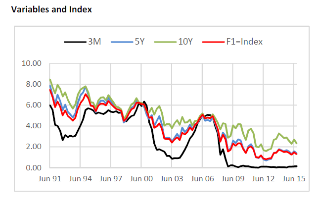
Application of the PCA analysis is illustrated for the samples of US$ Treasury yield rates with 3-month, 5-year, and 10-year maturity terms. The movements in the interest rates with different maturities are typically strongly correlated and therefore multiple series of interest rates with different maturities can be replaced with a single series that represents the market. The movement in each individual series can be decomposed into the common factor that represents the movement in the market and individual factor that represents the change in the term premium.
Results of the analysis are presented below.
- Estimated matrices
Ω V 0.99 0.90 0.80 0.56 0.60 0.58 0.90 0.99 0.97 -0.79 0.17 0.59 0.80 0.97 0.99 -0.25 0.78 -0.57
and eigen-values: (2.77, 0.20, 0.003). Note that in the example the main principal component V(1) = (0.56, 0.60, 0.58) assigns almost equal weight to each of the maturity terms. Therefore the index series estimated based on PCA analysis is effectively equal to simple average of the yield series with different maturity terms.
- Data. The exhibit below shows the movement in the input interest rate
series and the movement in the main principal component that models the common
factor that determines the movement in each individual series.